If you need a customer lifetime value calculation, then a free Excel spreadsheet template is available for download here… free clv template download
Contents
How to use the customer lifetime value Excel template
When you open the spreadsheet, it should look like this…
You should notice that the steps are clearly labelled in yellow and that there are only four steps, as will be discussed below.
Step ONE in the free customer lifetime value Excel template
Input promotional/acquisition expenses and number of new customers
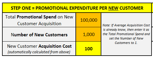
This will calculate the average new customer acquisition costs, as shown in below diagram:
In this step, you need to enter two numbers in the gold cells. The first number needed is the total promotional spend on new customer acquisition only. This may differ from the firm’s overall promotional expenditure, as they may also allocate funds for communicating to existing customers.
In the above example, an amount of $100,000 has been input. Directly under that number, you need to input the number of new customers acquired. In this example, we have used 1,000 new customers. The new customer acquisition cost is then automatically calculated.
As it says in the note on the side, if you already know the average acquisition cost, then simply enter it as the total promotional spend and then set the number of new customers to 1.
Step TWO when using the CLV Excel template
Choose and enter an appropriate discount rate
Step two is an optional, but recommended, step in the calculation of customer lifetime value. Most firms will have an average return on their investments, or possibly use a hurdle rate to evaluate new investment opportunities – this rate should be used.
If this is not available, usually as a rate of 10 to 20% is appropriate depending upon the investment return required. Please review articles on discount rates.
Step THREE in the free customer lifetime value Excel template
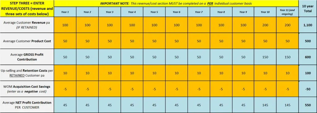
Enter customer revenues and customer costs – on a PER customer basis
As you can see from the above diagram, there are four rows to complete – the first is customer revenues, which is the total income received from the average customer across all products and services.
The average customer product cost (underneath) is the variable cost required to provide those products and services to the average customer.
The first row of the customer revenue less the average customer product costs automatically calculates the gross profit contribution per customer each year (in the first blue row).
Underneath the gross profit contribution there are two more rows of costs. The first is for any loyalty/retention costs and any up selling costs. Basically, these are the costs of marketing investments aimed at existing customers in order to grow and hold the business.Please refer to the article on retention goals.
The final row is actually a cost saving – which is appropriate to use when the brand has supporting customers that refer new business (non-customers) – so word-of-mouth (WOM) actually saves the firm money by reducing acquisition costs. Please refer to the article on word-of-mouth cost savings.
Step FOUR in the free customer lifetime value Excel template
Determine and enter the annual customer retention rate
For the fourth step in using the free CLV template, you only need to enter the annual customer retention (or loyalty) rate. The customer lifetime in years is then automatically calculated for you. It is more likely that a firm would know its retention or loyalty rate, rather than its lifetime period (in years) for customers.
A formula can generally be used to calculate the second number. The formula is 1/(1 – retention rate). For example, if the retention rate was 80%, then the formula would be 1/(1-0.8) = 1/0.2 = 5 years.
In the spreadsheet calculation, customer retention rate is used as an estimate of probability of receiving the future customer cash flows (that is, revenues and costs).
Related Topics
Why customer revenue will increase over time
A video on using the customer lifetime value template
Understanding customer lifetime value


